heormodel

Author

Pedro Nascimento de Lima

Health economic evaluation in Python: parameter sampling, simulation across model types, cost-effectiveness analysis, and value-of-information analysis for model-based health technology assessment.

Install

pip install heormodel

The calibration extra adds Bayesian calibration: pip install "heormodel[calibration]".

Quickstart

This example builds a three-state Markov cohort state-transition model comparing standard care with two treatments of different efficacy and cost, then evaluates it by probabilistic sensitivity analysis:

import matplotlib.pyplot as plt
import numpy as np
import pandas as pd
from heormodel.models import CohortSpec, MarkovModel
from heormodel.params import Beta, Gamma, ParameterSet
from heormodel.run import SeedManager, run_psa
from heormodel.cea import ceac, ceaf, icer_table
from heormodel.report import plot_ce_plane, plot_ceac
from heormodel.voi import evpi

WTP = 50_000.0


def model(p, intervention):
    rr = {"Standard care": 1.0, "Treatment A": p["rr_a"], "Treatment B": p["rr_b"]}[intervention]
    add_cost = {"Standard care": 0.0, "Treatment A": p["c_a"], "Treatment B": p["c_b"]}[intervention]
    p_progress = p["p_progress"] * rr
    # Transition matrix. Rows: current state. Columns: next state.
    P = np.array([
        [1 - p_progress - p["p_die"], p_progress, p["p_die"]],
        [0.0, 1 - p["p_die_sick"], p["p_die_sick"]],
        [0.0, 0.0, 1.0],
    ])
    cost = np.array([0.0, p["c_sick"], 0.0])
    cost[:2] += add_cost
    return CohortSpec(P, cost, np.array([1.0, p["u_sick"], 0.0]))


engine = MarkovModel(states=("Healthy", "Sick", "Dead"),
                     interventions=("Standard care", "Treatment A", "Treatment B"),
                     transitions_and_rewards=model, n_cycles=40)

params = ParameterSet({
    "p_progress": Beta(20, 180), "rr_a": Beta(75, 25), "rr_b": Beta(45, 55),
    "p_die": Beta(5, 995), "p_die_sick": Beta(50, 450),
    "c_sick": Gamma(100, 250.0), "c_a": Gamma(100, 20.0), "c_b": Gamma(100, 110.0),
    "u_sick": Beta(150, 50),
})

draws = params.sample(2_000, seed=SeedManager(1).generator())
outcomes = run_psa(engine, draws).outcomes
icer_table(outcomes).round(1)
cost effect inc_cost inc_effect icer status
intervention
Standard care 142239.3 11.2 NaN NaN NaN ND
Treatment A 155820.7 12.4 13581.4 1.2 10995.9 ND
Treatment B 272260.5 14.7 116439.7 2.2 51770.1 ND

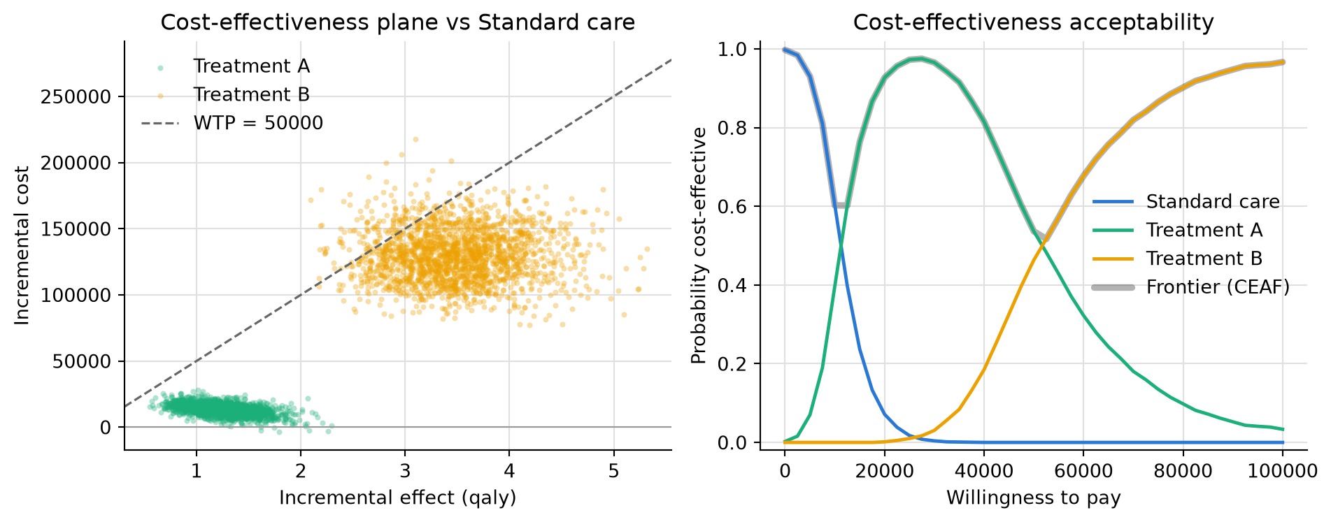
The icer_table orders interventions by cost and reports incremental cost-effectiveness ratios along the efficiency frontier; the status column flags dominated (D) and extended-dominated (ED) interventions. All three interventions sit on the frontier here, with Treatment A entering near 11,000 per quality-adjusted life-year (QALY) and Treatment B near 52,000. plot_ce_plane scatters every iteration’s incremental cost and effect against standard care, and plot_ceac reports the share of iterations in which each intervention has the highest net benefit, across a grid of willingness-to-pay thresholds:

grid = np.linspace(0, 100_000, 41)
ceac_df = ceac(outcomes, grid)
ceaf_df = ceaf(outcomes, grid)

fig, axes = plt.subplots(1, 2, figsize=(10, 4))
plot_ce_plane(outcomes, comparator="Standard care", wtp=WTP, ax=axes[0])
plot_ceac(ceac_df, ceaf_df=ceaf_df, ax=axes[1])
fig.tight_layout()

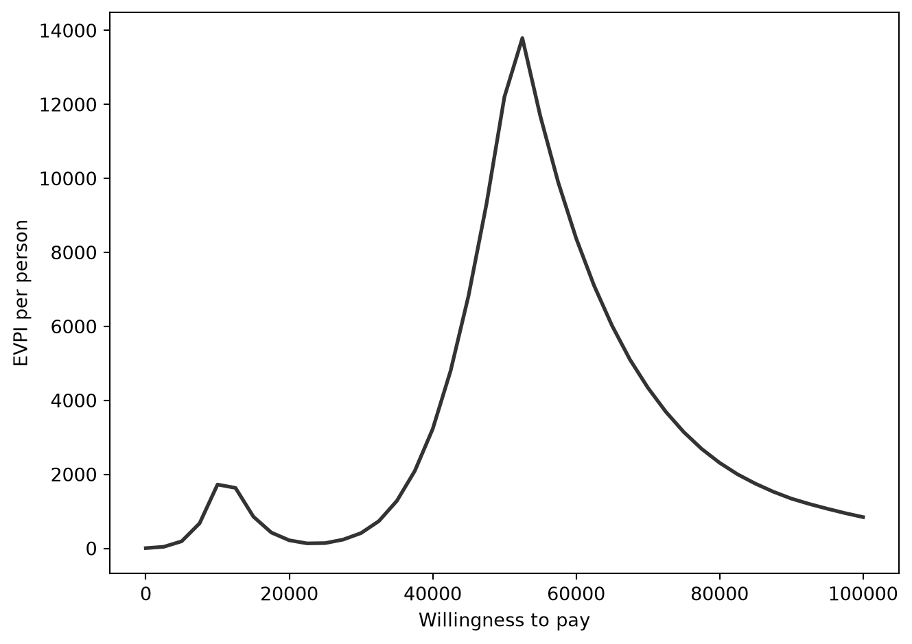
At a willingness-to-pay threshold of 50,000, the acceptability curves cross: the choice between Treatment A and Treatment B is close, so the expected value of perfect information (EVPI) is high there. Swept across the threshold, EVPI peaks near each ICER on the frontier, sharpest where the decision is closest:

evpi_curve = evpi(outcomes, grid)
print(f"EVPI at WTP {WTP:,.0f}: {evpi(outcomes, WTP):,.1f}")

fig2, ax2 = plt.subplots()
ax2.plot(grid, evpi_curve.to_numpy(), color="#333333", lw=2)
ax2.set_xlabel("Willingness to pay")
ax2.set_ylabel("EVPI per person")
fig2.tight_layout()
EVPI at WTP 50,000: 12,205.0

Where to go next

  • Markov cohort model: the standard state-transition model, then the microsimulation engine as the step up in detail.
  • Compartmental transmission model: a susceptible-exposed-infectious-recovered vaccination model written as ordinary differential equations, for infectious-disease cost-effectiveness analysis.
  • Bring your own outputs: an external results table through cost-effectiveness analysis, value of information, plots, and a run report.
  • Full pipeline: parameters, run_psa, cost-effectiveness analysis, and value of information end to end.
  • Calibration workflow: calibrate some parameters, take the rest from the literature, mix both with mix_draws, then run the same analyses.
  • API reference: every public function, generated from docstrings.
  • Changelog: what has shipped.