Deterministic sensitivity analysis

Probabilistic sensitivity analysis answers how uncertain a decision is; deterministic sensitivity analysis (DSA) instead answers which parameters move the result, and by how much. This tutorial shows how to run the three standard DSA designs, one-way, one-at-a-time, and grid, on the same Sick-Sicker cohort model the cohort tutorial uses for its probabilistic analysis, so the two are worth reading as a pair. The full script is examples/dsa.py.

heormodel.dsa builds scenario designs that run through run_psa like any draw matrix: a design has one row per scenario instead of one row per random draw, paired with a descriptor naming what each scenario varied. The same cost-effectiveness functions then read the outcomes, so a deterministic analysis reuses everything a probabilistic one does.

Specifying the model and base case

The model is the four-state Sick-Sicker cohort of the cohort tutorial. The base case is its Table 1 point estimates, held in a pandas.Series indexed by parameter name, the input every DSA builder takes.

import numpy as np
import pandas as pd
from heormodel.models import CohortSpec, MarkovModel

STATES = ("H", "S1", "S2", "D")
INTERVENTIONS = ("Standard of care", "Intervention A", "Intervention B", "Intervention AB")

def r2p(rate):
    return 1.0 - np.exp(-np.asarray(rate))

def model(p, intervention):
    p_HS1, p_S1H, p_S1S2 = r2p(p["r_HS1"]), r2p(p["r_S1H"]), r2p(p["r_S1S2"])
    p_HD, p_S1D, p_S2D = r2p(p["r_HD"]), r2p(p["r_HD"] * p["hr_S1"]), r2p(p["r_HD"] * p["hr_S2"])
    prog = r2p(p["r_S1S2"] * p["hr_S1S2_trtB"]) if "B" in intervention else p_S1S2
    P = np.zeros((4, 4))
    P[0, 0], P[0, 1], P[0, 3] = (1 - p_HD) * (1 - p_HS1), (1 - p_HD) * p_HS1, p_HD
    P[1, 0], P[1, 2], P[1, 3] = (1 - p_S1D) * p_S1H, (1 - p_S1D) * prog, p_S1D
    P[1, 1] = (1 - p_S1D) * (1 - p_S1H - prog)
    P[2, 2], P[2, 3], P[3, 3] = 1 - p_S2D, p_S2D, 1.0
    add = {"Standard of care": 0.0, "Intervention A": p["c_trtA"],
           "Intervention B": p["c_trtB"], "Intervention AB": p["c_trtA"] + p["c_trtB"]}[intervention]
    cost = np.array([p["c_H"], p["c_S1"] + add, p["c_S2"] + add, 0.0])
    u_s1 = p["u_trtA"] if intervention in ("Intervention A", "Intervention AB") else p["u_S1"]
    return CohortSpec(P, cost, np.array([p["u_H"], u_s1, p["u_S2"], 0.0]))

engine = MarkovModel(states=STATES, interventions=INTERVENTIONS, transitions_and_rewards=model,
                     n_cycles=75, initial_state="H", cycle_correction="simpson")

base = pd.Series(dict(
    r_HD=0.002, r_HS1=0.15, r_S1H=0.5, r_S1S2=0.105, hr_S1=3.0, hr_S2=10.0,
    hr_S1S2_trtB=0.6, c_H=2000.0, c_S1=4000.0, c_S2=15000.0, c_trtA=12000.0,
    c_trtB=13000.0, u_H=1.0, u_S1=0.75, u_S2=0.5, u_trtA=0.95))
WTP = 100_000.0

Running a one-way sweep

one_way varies a single parameter across the listed values, holding the rest at base. The result runs through run_psa like any draw matrix. Here the incremental net monetary benefit of Intervention AB over standard of care falls as the treatment-B cost rises, crossing zero near its base value.

from heormodel.cea import nmb
from heormodel.dsa import one_way
from heormodel.run import run_psa

design, _ = one_way(base, "c_trtB", [8_000.0, 13_000.0, 18_000.0])
nb = nmb(run_psa(engine, design).outcomes, WTP)
(nb["Intervention AB"] - nb["Standard of care"]).round(0)

iteration
0    65162.0
1    15256.0
2   -34650.0
dtype: float64

Building a one-at-a-time tornado

one_at_a_time sweeps each parameter between its low and high in turn, the union of one-way sweeps with the base case included once. tornado_data reads the (design, descriptor) pair directly, taking the net monetary benefit at each parameter’s low and high value. It returns the same table its probabilistic form does, so plot_tornado is unchanged.

from heormodel.dsa import one_at_a_time
from heormodel.report import plot_tornado, tornado_data

ranges = {name: (0.8 * base[name], 1.2 * base[name]) for name in base.index}
oat = one_at_a_time(base, ranges)
td = tornado_data(run_psa(engine, oat[0]).outcomes, oat, wtp=WTP,
                  intervention="Intervention AB", comparator="Standard of care")
plot_tornado(td.head(6))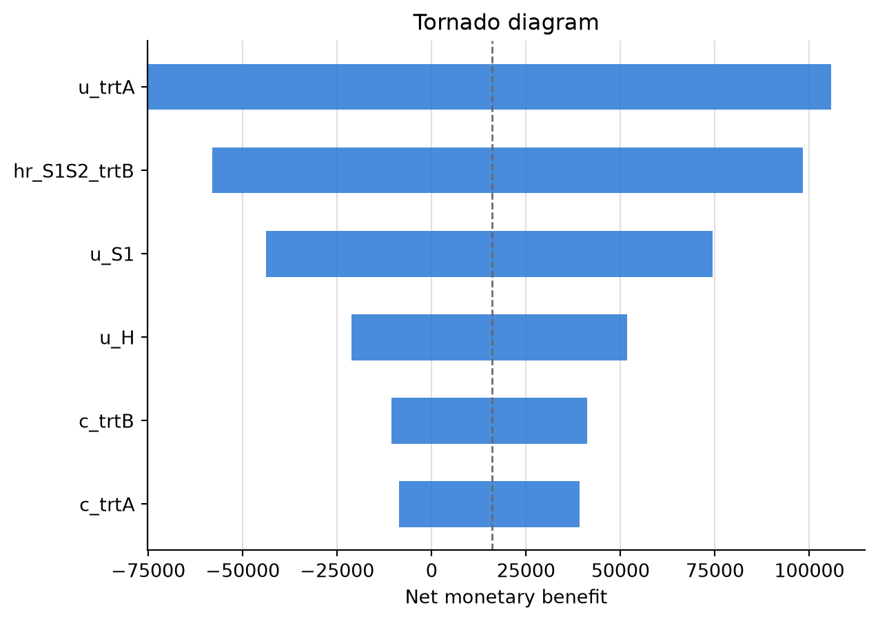

The utility of the treated Sick state (u_trtA) and the progression hazard ratio under treatment B (hr_S1S2_trtB) move the result most; the state costs barely register.

Sweeping a two-way grid

grid takes the full factorial of two or more parameters. heatmap_data reshapes a per-scenario outcome into a matrix over two of them. Here the incremental net monetary benefit of Intervention AB spans positive to negative across the two treatment costs.

from heormodel.dsa import grid
from heormodel.report import heatmap_data

gd, gdesc = grid(base, {"c_trtA": [6_000.0, 12_000.0, 18_000.0],
                        "c_trtB": [8_000.0, 13_000.0, 18_000.0]})
gnb = nmb(run_psa(engine, gd).outcomes, WTP)
heatmap_data(gnb["Intervention AB"] - gnb["Standard of care"], gdesc,
             x="c_trtA", y="c_trtB").round(0)

c_trtA	6000.0	12000.0	18000.0
c_trtB
8000.0	125049.0	65162.0	5275.0
13000.0	75143.0	15256.0	-44631.0
18000.0	25237.0	-34650.0	-94538.0

The grid center reproduces the one-way sweep’s base value, since both hold the other parameters at base. Where the probabilistic analysis integrates over the joint distribution, the deterministic analysis holds everything else fixed and reads one axis at a time.

Next: the replication gallery collects the published models these engines reproduce.