Full pipeline

This tutorial shows how to run the standard probabilistic sensitivity analysis workflow end to end: specify parameters, sample draws, evaluate a model with run_psa, then feed the outcomes to cost-effectiveness and value-of-information analysis. Bring your own outputs covers the analysis functions in more detail; here the focus is the run itself.

Specifying and sampling parameters

Distributions are specified directly or from published mean and standard error. ParameterSet.sample returns a draw matrix, one row per iteration; a Spearman rank correlation can be requested per parameter pair.

from heormodel.params import Beta, Gamma, Normal, ParameterSet
from heormodel.run import SeedManager

params = ParameterSet(
    {
        "p_event": Beta.from_mean_se(0.20, 0.03),
        "rr_treat": Normal(0.70, 0.10),
        "c_event": Gamma.from_mean_se(25_000, 3_000),
        "c_treat": Gamma.from_mean_se(4_000, 500),
        "u_event": Beta.from_mean_se(0.65, 0.05),
    }
)
seeds = SeedManager(42)
draws = params.sample(4_000, seed=seeds.generator())
draws.head(3).round(3)

	p_event	rr_treat	c_event	c_treat	u_event
iteration
0	0.208	0.596	27193.206	4466.640	0.550
1	0.162	0.713	23945.992	3970.817	0.607
2	0.226	0.778	25078.163	4567.860	0.674

Writing the model as a function

A model is a function that takes the draw matrix and returns Outcomes. The one below is a two-intervention decision tree evaluated over one year. Outcomes.from_wide builds that result from per-intervention cost and effect columns.

import pandas as pd
from heormodel.models import Outcomes

def decision_tree(d: pd.DataFrame) -> Outcomes:
    p_treated = d["p_event"] * d["rr_treat"]
    costs = pd.DataFrame({
        "No treatment": d["p_event"] * d["c_event"],
        "Treatment": d["c_treat"] + p_treated * d["c_event"],
    })
    effects = pd.DataFrame({
        "No treatment": 1 - d["p_event"] * (1 - d["u_event"]),
        "Treatment": 1 - p_treated * (1 - d["u_event"]),
    })
    return Outcomes.from_wide(costs, effects)

Running the probabilistic sensitivity analysis

run_psa evaluates the model on every draw and keeps each outcome matched to the parameters that produced it, the link value-of-information analysis relies on. It runs in parallel by default; this run is small, so sequential=True runs it without that overhead.

from heormodel.run import run_psa

outcomes = run_psa(decision_tree, draws, sequential=True).outcomes
outcomes.summary().round(3)

	cost	qaly
intervention
No treatment	4986.265	0.930
Treatment	7505.804	0.951

Analyzing cost-effectiveness and value of information

Nothing from here on is specific to a decision tree: the same icer_table, evpi, and evppi_ranking calls apply to the Outcomes any model produces.

import numpy as np
from heormodel.cea import icer_table
from heormodel.voi import evpi, evppi_ranking

icer_table(outcomes).round(3)

	cost	effect	inc_cost	inc_effect	icer	status
intervention
No treatment	4986.265	0.930	NaN	NaN	NaN	ND
Treatment	7505.804	0.951	2519.54	0.021	121203.865	ND

Treatment is the more expensive, more effective intervention; whether its incremental cost-effectiveness ratio stays below a given willingness-to-pay threshold, and how much resolving that uncertainty would be worth, are what EVPI and the per-parameter ranking answer next.

WTP = 50_000.0
print(f"EVPI at WTP {WTP:,.0f}: {evpi(outcomes, WTP):,.2f}")
evppi_ranking(outcomes, draws, WTP).round(2)

EVPI at WTP 50,000: 47.03

rr_treat    9.75
p_event     0.70
c_treat     0.12
u_event     0.00
c_event     0.00
Name: evppi, dtype: float64

Checking convergence with running means

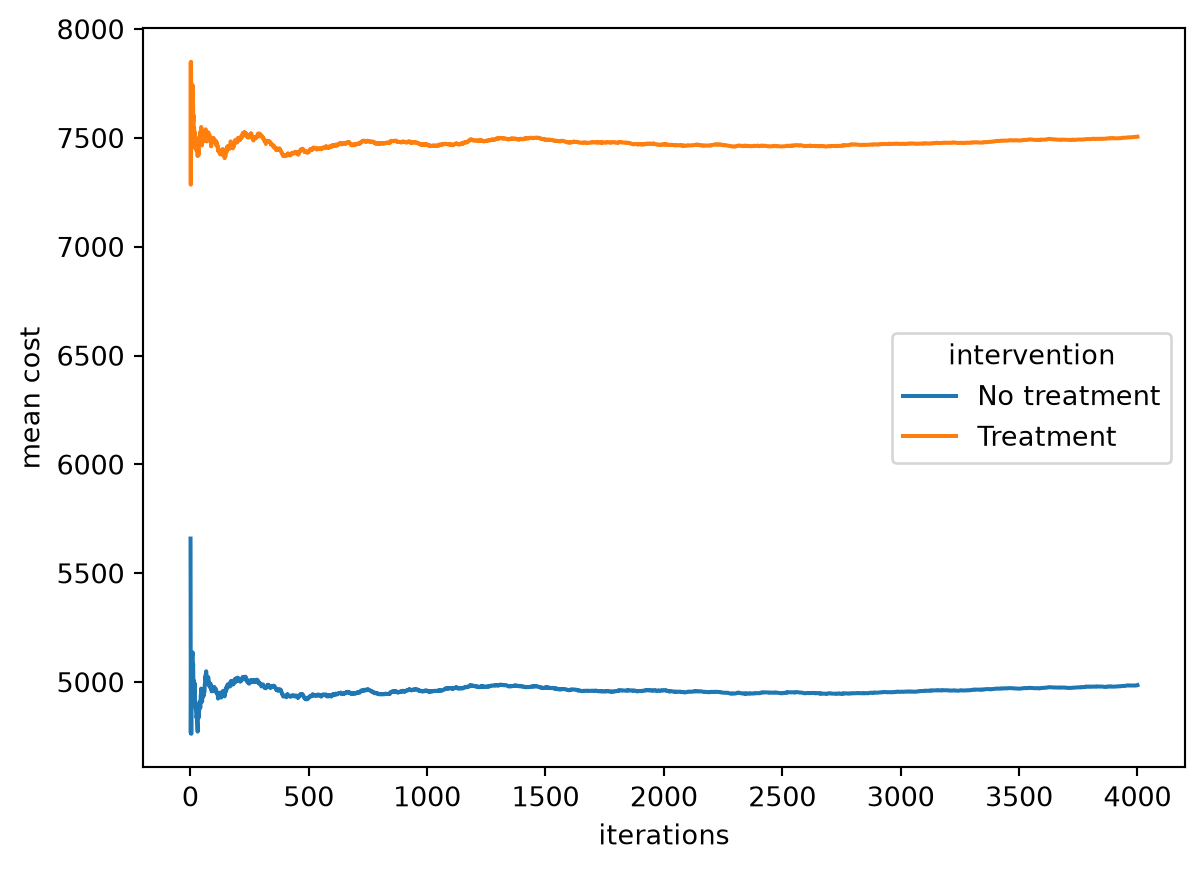
running_means tracks the running mean of an outcome column per intervention as iterations accumulate; flat traces at the right edge suggest the iteration count is adequate for the means (value-of-information estimates typically need more).

from heormodel.run import running_means

running_means(outcomes).plot(xlabel="iterations", ylabel="mean cost");

The engines concept page describes the model types run_psa can run. Next: the value of information tutorial takes outcomes like these through the expected value of perfect, partial perfect, and sample information, checking each against a closed form.