import numpy as np
import pandas as pd
from scipy.stats import norm
from heormodel.models import Outcomes
from heormodel.params import Normal, ParameterSet
from heormodel.run import run_psa

WTP = 30_000.0
MU_Q, SD_Q = 0.20, 0.30
MU_C, SD_C = 4_000.0, 8_000.0

def new_drug(d: pd.DataFrame) -> Outcomes:
    zero = np.zeros(len(d))
    costs = pd.DataFrame({"Standard care": zero, "New drug": d["dc"]}, index=d.index)
    effects = pd.DataFrame({"Standard care": zero, "New drug": d["dq"]}, index=d.index)
    return Outcomes.from_wide(costs, effects)

params = ParameterSet({"dq": Normal(MU_Q, SD_Q), "dc": Normal(MU_C, SD_C)})
draws = params.sample(100_000, seed=2026)
outcomes = run_psa(new_drug, draws, sequential=True).outcomesValue of information
This tutorial shows how to run the full value-of-information workflow, expected value of perfect information (EVPI), of partial perfect information (EVPPI), and of sample information (EVSI), and checks every estimate against a closed form, continuing from the full pipeline tutorial. The model is the Gaussian linear decision model that anchors the regression value-of-information literature (Strong, Oakley & Brennan, 2014, Medical Decision Making 34:311-326; Strong, Oakley, Brennan & Breeze, 2015, Medical Decision Making 35:570-583): its incremental net benefit is Normal, so all three measures have closed forms via the unit normal loss integral, which is what lets this page check each estimate rather than assume it. The measures follow the good-practice framing of Rothery and others (2020, Value in Health 23:277-286). The full script is examples/voi_tutorial.py.
Specifying the decision model
Two interventions, standard care and a new drug, differ by an uncertain incremental effect dq (quality-adjusted life-years, QALYs) and an uncertain incremental cost dc, both Normal. At a 30,000-per-QALY threshold the drug is cost-effective on the means, so value of information asks not which intervention to pick but the value of more evidence to reduce the decision uncertainty.
The closed forms use the unit normal loss integral: the value of resolving uncertainty is the expected upside minus the current decision’s value.
def emax0(m, s):  # E[max(0, X)] for X ~ Normal(m, s**2)
    return m * norm.cdf(m / s) + s * norm.pdf(m / s)

def analytic_voi(s_conditional):
    m = WTP * MU_Q - MU_C
    return emax0(m, s_conditional) - max(0.0, m)
EVPI: the ceiling on research value
EVPI is the difference between a decision made with perfect information and one made with current information, an upper bound on the value of any research. evpi recovers the closed form within Monte Carlo error.
from heormodel.voi import evpi

s_total = np.hypot(WTP * SD_Q, SD_C)
pd.Series({"estimate": evpi(outcomes, WTP), "closed form": analytic_voi(s_total)}).round(0)
estimate 3892.0
closed form 3870.0
dtype: float64EVPPI: which parameters carry that value
EVPPI is the value of resolving one parameter while the rest stay uncertain. It identifies which parameters drive the decision uncertainty, so evppi_ranking sweeps each and sorts them into a research priority list. The effect dq beats the cost dc here because WTP * SD_Q exceeds SD_C.
from heormodel.voi import evppi, evppi_ranking

ranking = evppi_ranking(outcomes, draws, WTP)
closed = pd.Series({"dq": analytic_voi(WTP * SD_Q), "dc": analytic_voi(SD_C)})
pd.DataFrame({"estimate": ranking, "closed form": closed}).round(0)| estimate | closed form | |
|---|---|---|
| dq | 2709.0 | 2679.0 |
| dc | 2313.0 | 2291.0 |
The ranking is threshold-specific: below about 28,000 per QALY the cost leads instead. The default spline metamodel suits one or two parameters; method="gp" (a Gaussian process) handles groups of many parameters.
EVSI: the value of a specific study
EVSI is the value of a study of finite sample size, not perfect resolution. Consider a two-arm trial measuring the incremental effect, each arm reporting a mean QALY difference with sampling standard deviation tau = 1 / sqrt(n). simulate_summaries draws one trial summary per parameter draw from its true dq, and evsi_regression reads the value off the fitted conditional means, checked here against the closed form.
from heormodel.voi import evsi_regression, simulate_summaries

tau = 1.0 / np.sqrt(200)
summaries = simulate_summaries(
    draws, lambda row, r: {"xbar": row["dq"] + r.normal(0.0, tau)}, seed=200)
s_evsi = WTP * SD_Q**2 / np.hypot(SD_Q, tau)
pd.Series({"estimate": evsi_regression(outcomes, summaries, WTP),
           "closed form": analytic_voi(s_evsi)}).round(0)
estimate 2615.0
closed form 2585.0
dtype: float64Reported against the willingness-to-pay threshold, EVSI is a family of curves, one per sample size. Each fans out between zero and the effect EVPPI, not the EVPI: this trial measures only the effect, so it cannot resolve the cost uncertainty, which stays in the decision and caps the study’s value below perfect information. A trial that also measured cost would climb toward EVPI instead. Larger trials shrink tau, lifting each curve toward its ceiling.
import matplotlib.pyplot as plt
from matplotlib import cm, colors

grid = np.linspace(0, 120_000, 13)
sizes = [25, 50, 100, 200, 400, 800]
rng = np.random.default_rng(0)
fan = {}
for n in sizes:  # the same study, evaluated across the threshold grid
    xbar = draws["dq"] + rng.normal(0.0, 1.0 / np.sqrt(n), len(draws))
    summ = pd.DataFrame({"xbar": xbar}, index=draws.index)
    fan[n] = [evsi_regression(outcomes, summ, k) for k in grid]

ramp, scale = plt.get_cmap("Purples"), colors.LogNorm(min(sizes), max(sizes))
fig, ax = plt.subplots()
for n in sizes:
    ax.plot(grid, fan[n], color=ramp(0.3 + 0.6 * scale(n)), lw=1.4)
ax.plot(grid, evpi(outcomes, grid).to_numpy(), color="#333333", lw=2, label="EVPI")
ax.plot(grid, [evppi(outcomes, draws, "dq", k) for k in grid],
        color="#eb6834", lw=2, label="EVPPI (effect)")
ax.set(xlabel="willingness to pay", ylabel="value per person")
ax.legend(loc="upper left")
sm = cm.ScalarMappable(norm=scale, cmap=ramp); sm.set_array([])
fig.colorbar(sm, ax=ax, label="trial size (n per arm)");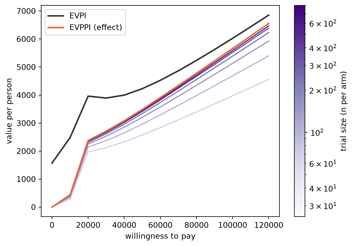
Two features look odd until you read them off the model. At a zero threshold EVPI is already about 1,600: health is unpriced, so the choice turns on cost alone, and the uncertain cost dc is a saving 31% of the time that perfect information would capture. The EVSI curves start at zero there, since an effect study is worthless when the effect has no value. And nothing peaks: the net benefit standard deviation hypot(WTP * SD_Q, SD_C) grows with the threshold, so the stakes of a wrong choice climb while the chance of one settles near 25%. A model with bounded outcome variance would grow certain at a high threshold instead, its value of information peaking near the tie then decaying.
Expected net benefit of sampling
Per-person EVSI becomes a funding decision once scaled to the population it informs. Multiply by the beneficiary population, 2,000 patients a year over 10 years discounted at 3.5%, then subtract the study cost, a 300,000 setup plus 6,000 per participant (two arms, so 2n). The difference is the expected net benefit of sampling (ENBS), and ENBS at or above zero is the condition for running the study. It peaks at an interior size: smaller is underpowered, larger buys less EVSI than it costs.
i30 = int(np.where(grid == WTP)[0][0])
evsi = pd.Series({n: fan[n][i30] for n in sizes})  # EVSI at the reference threshold
years = np.arange(10)
beneficiaries = 2_000 * (1.035 ** -years).sum()  # discounted future patients
cost = 300_000 + 6_000 * 2 * np.array(sizes)  # 2n participants
enbs = pd.Series(beneficiaries * evsi.to_numpy() - cost, index=pd.Index(sizes, name="n per arm"))
best = enbs.idxmax()
print(f"optimal size: {best} per arm, ENBS {enbs[best]:,.0f}")
enbs.round(0)
optimal size: 200 per arm, ENBS 42,290,935n per arm
25 35946386.0
50 39959462.0
100 42069547.0
200 42290935.0
400 40775364.0
800 36246797.0
dtype: float64ax = enbs.plot(marker="o", xlabel="trial size (n per arm)", ylabel="ENBS")
ax.axhline(0, color="0.6", lw=0.8);
ax.plot(best, enbs[best], "r*", ms=14);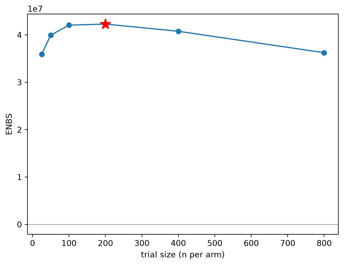
What these numbers say
EVPI is the ceiling: no research beats it. EVPPI ranks research targets, a ranking that shifts with the threshold. EVSI prices a concrete design against the uncertainty it can resolve, and ENBS weighs it against cost for a fund-or-not decision with a best sample size. Every estimate above lands within about one percent of its closed form at 100,000 iterations. Next: the calibration workflow feeds a calibrated posterior into the same pipeline.