Compartmental transmission model

This tutorial shows how to build an infectious-disease cost-effectiveness model with ODEModel, the engine for systems of ordinary differential equations, using a susceptible-exposed-infectious-recovered (SEIR) model of a vaccination program. A transmission model is what the cohort and microsimulation engines cannot express: the hazard a susceptible person faces is not fixed but rises and falls with how many others are infectious, so the compartments are coupled through a force of infection that changes over the course of the epidemic. Full script: examples/seir_vaccination.py.

Specifying the compartments and their dynamics

The model follows a closed population of 100,000 through an epidemic of a directly transmitted, non-fatal infection. Five compartments track the susceptible (S), the exposed but not yet infectious (E), the infectious (I), the recovered and immune (R), and the vaccinated and immune (V). The dynamics_and_rewards function returns an ODESpec: the right-hand side of the system (the rate of change of each compartment), the initial compartment sizes, and the reward rates. The force of infection is beta * I / N, where N is the living population and beta follows from the basic reproduction number, so a susceptible person’s rate of infection is proportional to the current infectious prevalence. Only the vaccination program vaccinates; the comparator sets the vaccination rate to zero, which is the branch-on-name pattern the engines share.

Rewards use the two channels the engine offers, matched to continuous time. Quality-adjusted life-years accrue on compartment occupancy through state_effect: everyone healthy contributes one per year and the infectious contribute less while ill, so averted illness raises the effect. Costs fall on flows rather than states: event_rates returns the per-year rate of two events, doses administered and new infections, and event_cost charges a one-time amount to each. The engine integrates the discounted reward flows alongside the compartments.

import numpy as np
import pandas as pd
from heormodel.models import ODEModel, ODESpec

STATES = ("S", "E", "I", "R", "V")
INTERVENTIONS = ("No vaccination", "Vaccination program")
POPULATION, INITIAL_INFECTIOUS = 100_000.0, 10.0

def seir(p, intervention):
    beta = p["R0"] * p["gamma"]  # transmission rate from the reproduction number
    nu = p["nu"] if intervention == "Vaccination program" else 0.0
    def derivatives(t, y):
        s, e, i, r, v = y
        foi = beta * i / (s + e + i + r + v)  # force of infection
        new_infections, doses = foi * s, nu * s
        return np.array([-new_infections - doses, new_infections - p["sigma"] * e,
                         p["sigma"] * e - p["gamma"] * i, p["gamma"] * i, doses])
    def event_rates(t, y):
        s, e, i, r, v = y
        foi = beta * i / (s + e + i + r + v)
        return np.array([nu * s, foi * s])  # doses per year, new infections per year
    return ODESpec(
        derivatives=derivatives,
        initial=np.array([POPULATION - INITIAL_INFECTIOUS, 0.0, INITIAL_INFECTIOUS, 0.0, 0.0]),
        state_cost=np.zeros(5), state_effect=np.array([1.0, 1.0, p["u_I"], 1.0, 1.0]),
        event_rates=event_rates,
        event_cost=np.array([p["c_vacc"], p["c_case"]]), event_effect=np.zeros(2))

engine = ODEModel(states=STATES, interventions=INTERVENTIONS,
                  dynamics_and_rewards=seir, horizon=10.0, discount_rate=0.03)

Reading the epidemic curves

trajectory integrates the compartments for one parameter set and returns them over time, which is useful for inspecting the model before trusting its cost-effectiveness output. Plotting the two arms side by side shows what the program does: without vaccination the susceptible pool is drawn down by infection, producing a wave of recovered individuals, while under the program susceptibles move to the vaccinated compartment before the epidemic can take hold, and the infectious wave never builds.

import matplotlib.pyplot as plt

base = pd.Series(dict(R0=1.8, sigma=4.0, gamma=6.0, nu=1.0, c_vacc=200.0, c_case=150.0, u_I=0.7))
no_vacc, vacc = engine.trajectory(base, "No vaccination"), engine.trajectory(base, "Vaccination program")

fig, axes = plt.subplots(1, 2, figsize=(9.5, 3.6), sharey=True)
for ax, traj, title in ((axes[0], no_vacc, "No vaccination"), (axes[1], vacc, "Vaccination program")):
    for comp in ("S", "I", "R", "V"):
        ax.plot(traj["time"], traj[comp], label=comp)
    ax.set_title(title); ax.set_xlabel("Year")
axes[0].set_ylabel("People"); axes[1].legend(loc="center right")
plt.show()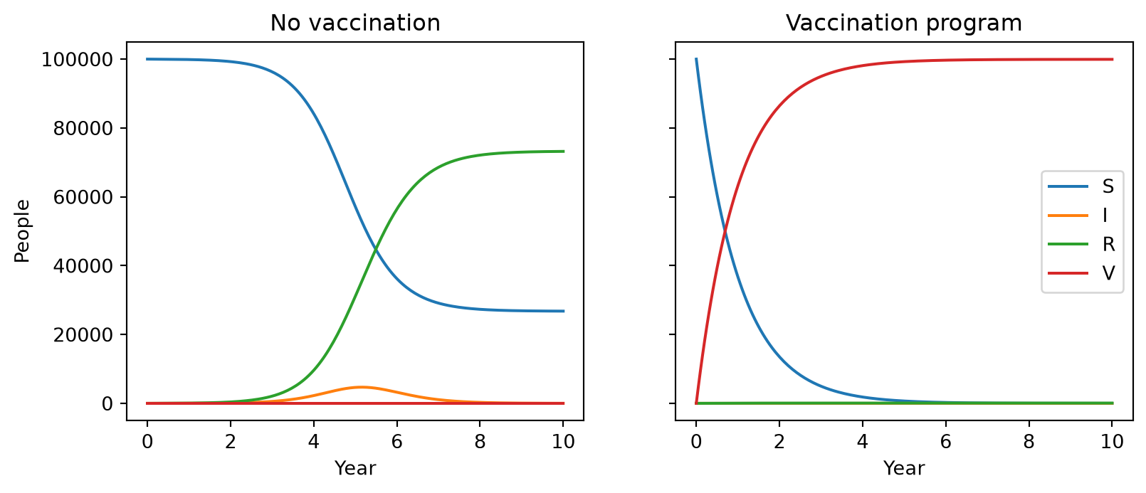

Vaccination cuts the total number ever infected over the ten-year horizon from about 73,000 to under 100, nearly eliminating the epidemic.

The base-case cost-effectiveness result

Integrating each arm once at the point estimates gives the deterministic cost-effectiveness result. Vaccination is not cost-saving here: it costs more than the treatment it averts, because the doses reach nearly everyone while the treatment cost per infection is modest. It is cost-effective, buying the quality-adjusted life-years from averted illness at an incremental cost-effectiveness ratio around 3,200 per quality-adjusted life-year, far below a 50,000 threshold.

from heormodel.cea import icer_table
draws0 = pd.DataFrame([base.to_dict()], index=pd.RangeIndex(1, name="iteration"))
icer_table(engine.evaluate(draws0)).round(2)

	cost	effect	inc_cost	inc_effect	icer	status
intervention
No vaccination	9512537.48	860808.38	NaN	NaN	NaN	ND
Vaccination program	19412280.17	863935.86	9899742.69	3127.48	3165.41	ND

Running the probabilistic sensitivity analysis

The epidemic and cost parameters become a ParameterSet; the reproduction number, rates, and costs take log-normal distributions that keep them positive, and the infectious-state utility takes a beta distribution bounded to the unit interval. The reproduction number carries the widest spread because it is the least certain and, as the value-of-information analysis shows, the most consequential. From there the analysis is identical to any other engine’s.

from heormodel.params import Beta, LogNormal, ParameterSet
from heormodel.run import SeedManager, run_psa

params = ParameterSet({
    "R0": LogNormal(np.log(1.8), 0.30), "sigma": LogNormal(np.log(4.0), 0.1),
    "gamma": LogNormal(np.log(6.0), 0.1), "nu": LogNormal(np.log(1.0), 0.15),
    "c_vacc": LogNormal(np.log(200.0), 0.25), "c_case": LogNormal(np.log(150.0), 0.25),
    "u_I": Beta(8.4, 3.6)})
draws = params.sample(1000, seed=SeedManager(20260711).generator())
outcomes = run_psa(engine, draws).outcomes
icer_table(outcomes).round(2)

	cost	effect	inc_cost	inc_effect	icer	status
intervention
No vaccination	8547209.69	861130.58	NaN	NaN	NaN	ND
Vaccination program	20001324.57	863933.24	11454114.88	2802.66	4086.87	ND

What the uncertainty is worth resolving

The cost-effectiveness acceptability curve reports, at each willingness-to-pay threshold, the probability that each arm is the better value across the draws. Vaccination becomes the preferred arm once the threshold passes its incremental cost-effectiveness ratio, and the crossover is where the two curves meet.

from heormodel.cea import ceac
from heormodel.report import plot_ceac
plot_ceac(ceac(outcomes, np.linspace(0, 30_000, 61)))
plt.show()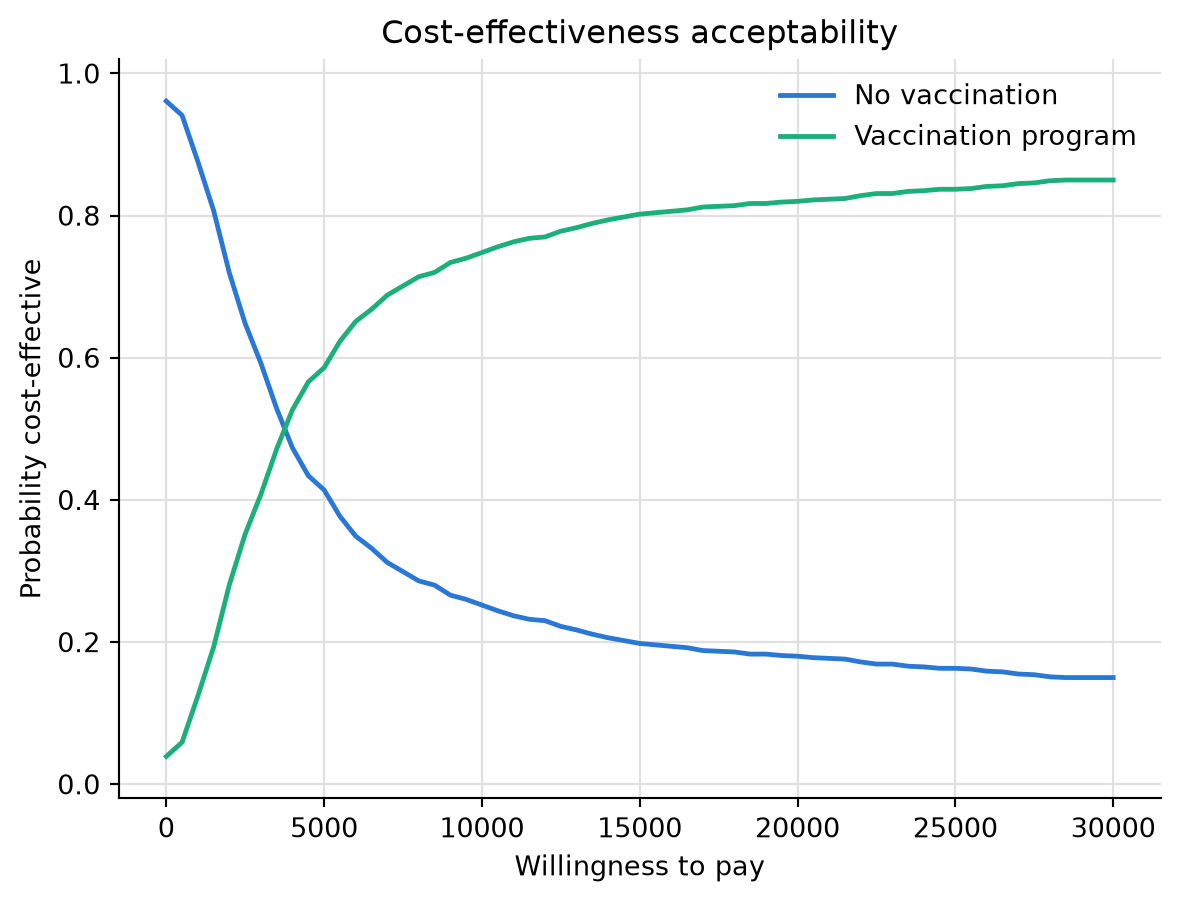

The expected value of perfect information measures what remains at stake at a given threshold. It is positive at 50,000 because the decision is not the same in every draw: when the reproduction number is low the outbreak is small, few infections are there to avert, and the program does not earn back its dose cost, so no vaccination is the better choice in those draws.

from heormodel.voi import evpi, evppi_ranking
print(f"EVPI at WTP 50,000: {evpi(outcomes, 50_000.0):,.0f}")

EVPI at WTP 50,000: 1,938,103

Partitioning that value across the parameters confirms where it lives. The expected value of partial perfect information ranks the reproduction number far above every other parameter, at a partial value on the order of the overall expected value of perfect information itself; both are regression estimates, so the partial value can land a little above the total. Resolving how transmissible the pathogen is would remove essentially all of the decision uncertainty, because it determines how large the averted epidemic would have been.

evppi_ranking(outcomes, draws, 50_000.0).round(0).head()

R0        2358086.0
u_I             0.0
c_case          0.0
gamma           0.0
sigma           0.0
Name: evppi, dtype: float64

Where this fits

The ordinary differential equation engine adds transmission dynamics to the engine set, alongside the cohort, microsimulation, and discrete-event engines. Because it returns the same Outcomes structure, the cost-effectiveness and value-of-information analysis is the code you already know. The engine is deterministic: one parameter set gives one epidemic trajectory. A stochastic counterpart, where the epidemic can fade out by chance in a small population, is planned as a follow-up.